2D Plane Stress Analysis with SymPy and ANSYS APDL
by Anıl ODABAŞ
Although, computers get stronger day by day, time is still precious to all of us. Thus, we need to simplify our Finite Element Analysis (FEA) as an engineer. 2D Plane Stress and Strain Analysis are very useful analysis types because of simplicty, speed and accuracy for the suitable model geometries, If the correct definitions are made. Finite Element Method means linear algebra. There are so many programmes for linear algebra such as Matlab, Mathematica etc. There is also a very powerful and easy and free Python module, right here. It’s name is SymPy, which is a very useful module for symbolic mathematics and linear algebra.
I would like to show an example of Daryl L. Logan’s comprehensive book “A First Course in the Finite Element Method”. A thin plate subjected to the surface traction shown in Figure.1, determine the nodal displacements and the element stresses. The plate thickness t = 1 in, E = 30.106 psi and ν = 0.30. Although, writer doesn’t indicate type of material, one can understand material type from Young’s modulus. Yes, it is steel.
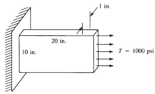
In this example, we just calculate nodal displacement with the help of SymPy. First of all, one must import SymPy module as a “sym”. If you don’t have SymPy library on your computer, you can install by typing pip install sympy command.
import sympy as sym
Also, should have to determine our symbols that we use in calculation.
Bi, Bn, Bm, gi, gn, gm, eta = sym.symbols("beta_i beta_n beta_m gamma_i gamma_n gamma_m eta")
And we need to assign variable.
E = 30 * (10 ** 6)  # Young Modulus of Steel in terms of psi
v = 0.3  # Poisson Ratio of Steel
t = 1  # Thickness of Section in.
q = 1000  # Pressure psi.
l = 20  # Length of Section in.
b = 10  # Width of Section in.
First of all, one have to discretize the plate. We discretize this plate into two elements for simplicity (Figure.2). A distributed load act on element can be concentrated at the nodes by using constant-strain triangle (CST).
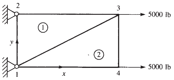
A = t * b
F = 0.5 * (q * A)

Nodes = sym.Matrix([[0, 0], [0, b], [l, b], [l, 0]])
Forces = sym.Matrix([F, 0, F, 0])
One can create matrix by using sympy as you can see codes given above. Now, we create stiffness matrices of elements that divided.
\begin{equation} [k] = t\cdot A\cdot[B]^T \cdot[D]\cdot[B] \end{equation}
In the famous algebric equation given above, [B] is a gradient matrix and [D] is a constitutive matrix. [B] changes with element size. [D] changes with material behaviour and many of things. In this case, we use linear material model for plane stress conditions.
A is the area of element that divided. We can easly create element from [Nodes] and calculate area of element.
Nodes1 = Nodes[:3, :2]
Area1 = sym.det(Nodes1.col_insert(1, sym.ones(3, 1))) * 0.5
Now, ready to create matrix B and matrix D for element one.
# [B] Matrix
Bi = Nodes1[2, 1] - Nodes1[1, 1]
Bn = Nodes1[1, 1] - Nodes1[0, 1]
Bm = Nodes1[0, 1] - Nodes1[2, 1]
gi = Nodes1[1, 0] - Nodes1[2, 0]
gn = Nodes1[0, 0] - Nodes1[1, 0]
gm = Nodes1[2, 0] - Nodes1[0, 0]

BI = (1 / (2 * Area1)) * sym.Matrix([[Bi, 0], [0, gi], [gi, Bi]])
BN = (1 / (2 * Area1)) * sym.Matrix([[Bn, 0], [0, gn], [gn, Bn]])
BM = (1 / (2 * Area1)) * sym.Matrix([[Bm, 0], [0, gm], [gm, Bm]])

B1 = sym.Matrix([[BI, BN, BM]])

# [D] Matrix
D = (E / (1 - v ** 2)) * sym.Matrix([[1, v, 0], [v, 1, 0], [0, 0, (1 - v) / 2]])
As you know, there are several ways to create matrix B, such as using for loop. But today, I am gonna show SymPy library abilities and some linear algebric manipulations. Here, we able to create stiffness matrix [k].
k1 = (t * Area1 * B1.T * D * B1)
We can reach matrix dimension with help of k1.shape. We have 3 nodes then stiffness matrix dimension is 6x6. Did you realise something? Yes, right. Global stiffness matrix [K] must be in 8x8 dimensions because of 4 number key nodes. Now, we arrange our stiffness matrix by adding zero matrix and also rotating the nodes counterclockwise direction.
k1.row_swap(2, 4)
k1.row_swap(3, 5)
k1.col_swap(4, 2)
k1.col_swap(5, 3)
K1 = (k1.row_join(sym.zeros(6, 2))).col_join(sym.zeros(2, 8))
We have to same loop for element two to get stiffness matrix.
Nodes2 = Nodes[1:4, :2]
Area2 = sym.det(Nodes2.col_insert(1, sym.ones(3, 1))) * 0.5

# [B] Matrix

Bi = Nodes2[2, 1] - Nodes2[1, 1]
Bm = Nodes2[1, 1] - Nodes2[0, 1]
Bn = Nodes2[0, 1] - Nodes2[2, 1]
gi = Nodes2[1, 0] - Nodes2[2, 0]
gn = Nodes2[0, 0] - Nodes2[1, 0]
gm = Nodes2[2, 0] - Nodes2[0, 0]

BI = (1 / (2 * Area2)) * sym.Matrix([[Bi, 0], [0, gi], [gi, Bi]])
BN = (1 / (2 * Area2)) * sym.Matrix([[Bn, 0], [0, gn], [gn, Bn]])
BM = (1 / (2 * Area2)) * sym.Matrix([[Bm, 0], [0, gm], [gm, Bm]])

B2 = sym.Matrix([[BI, BN, BM]])

# Stifffness Matrix of the Element-2
k2 = (t * Area2 * B2.T * D * B2)

k2.row_swap(2, 4)
k2.row_swap(3, 5)
k2.col_swap(4, 2)
k2.col_swap(5, 3)
K2 = (((k2.row_insert(2, sym.zeros(1, 6))).row_insert(2, sym.zeros(1, 6))).col_insert(2, sym.zeros(8, 1))).col_insert(2,sym.zeros(8,1))
Now, we can obtain global stiffness matrix of the system by superposing two matrices.
K = (K1 + K2)
Finally, we are able to obtain deformations on the nodes by equation given below.
\begin{equation} {F}=[K]{d} \end{equation}
d = ((K[0:4, 0:4]) ** -1) * Forces
sym.pprint(d * (10 ** 6))
You can display deformations on the terminal like below.
\[\left[\begin{array}{r} 609.6 \\ 4.2 \\ 663.7 \\ 104.1 \end{array}\right]\]Now it’s ANSYS Mechanical APDL turn. I tried to create macro file and i use PLANE42 element to build up the model. As you know, PLANE42 is old element but it is suitable to use for this question. May one use PLANE182 element.
/TITLE, 2D Plane Stress
FINISH
/CLEAR
/PREP7
/UNITS,BIN

BLC4,0,0,20,10

ET,1,PLANE42
KEYOPT,1,3,3

R,1,1

MP,EX,1,30e6
MP,PRXY,1,0.3


ESIZE,0,1


AMESH,ALL

FINISH

/SOLU
ANTYPE,0


DL, 4, ,ALL,0


SFL,2,PRES,-1000

SOLVE
FINISH

SAVE

/POST1

/WIND,ALL,OFF
/WIND,1,LTOP
/WIND,2,RTOP
/WIND,3,LBOT
/WIND,4,RBOT
GPLOT

/GCMD,1, PLDISP,2
/GCMD,2, PLNSOL,U,X,0,1
/GCMD,3, PLNSOL,U,Y,0,1
/GCMD,4, PLVECT,U,X
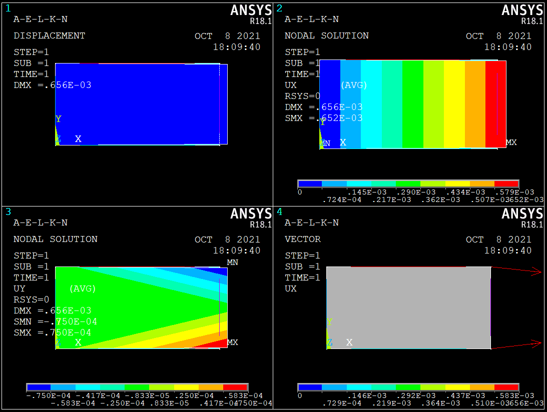
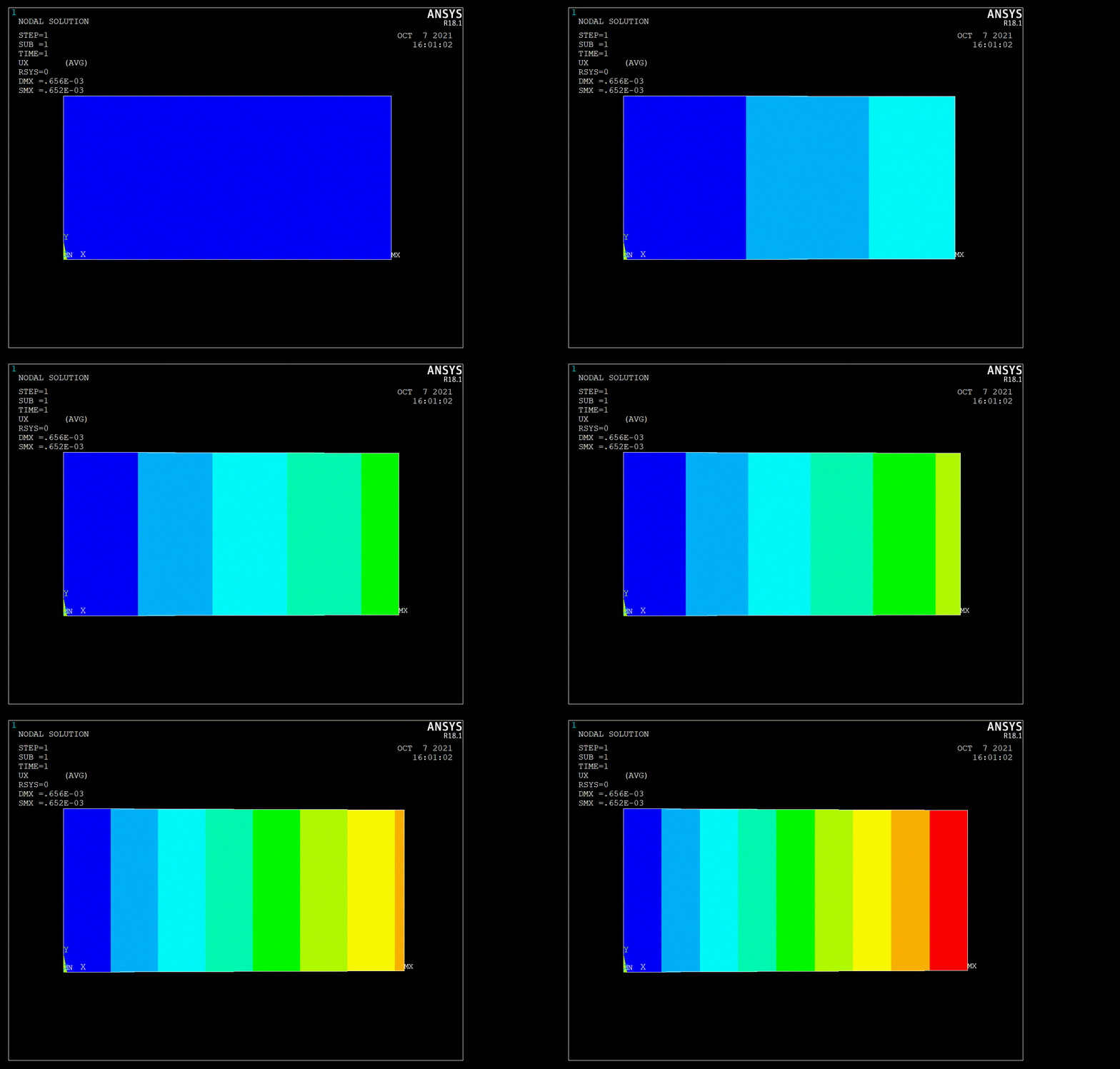
As can be seen in macro code given above, I didn’t mesh in triangular shape. If i use triangular shape for mesh, ANSYS would be create to node at the middle of the area. That’s why I didn’t mesh in tria shape. At the end of the analysis, I got some solution given below (Figure.3).
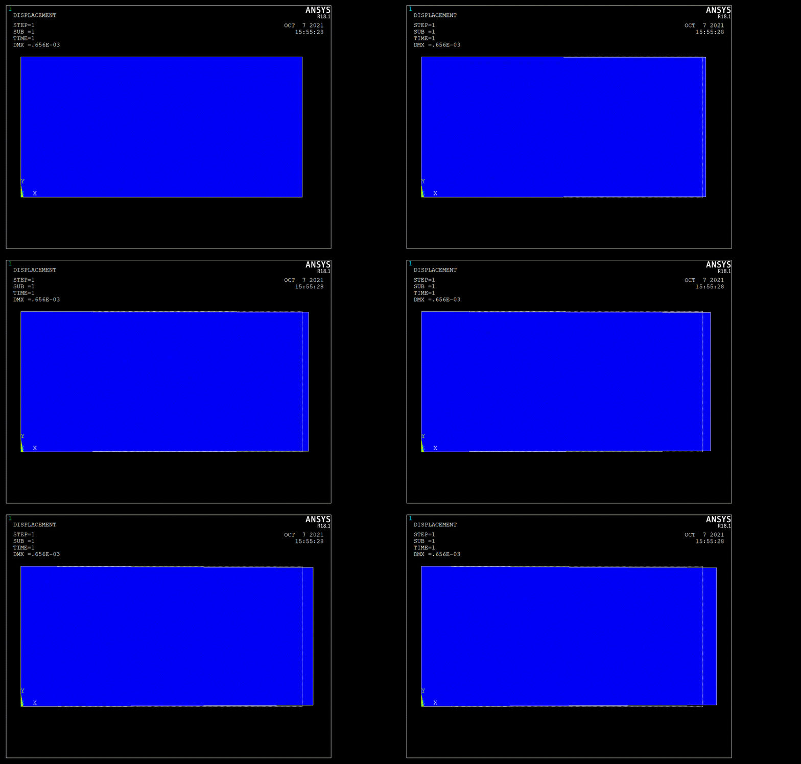
And of course, ANSYS’s indispensable animations.
A one-dimensional bar’s displacement subjected to tensile force can be calculated by the equation given below. \begin{equation} \delta=\frac{P L}{A E}=\frac{(10000) 20}{10\left(30 \times 10^{6}\right)}=670 \times 10^{-6} \text { in } \end{equation}
This result \(670 \cdot 10^{-6} \mbox{ in}\) can be first approximation as book’s says, ANSYS gives us \(656\cdot 10^{-6} \mbox{ in}\) and finally SymPy’s calculation \(663.70\cdot 10^{-6} \mbox{ in}\). Indeed, Finite Element Methods are powerfull methods for approximation to exact solution. Note that, FE Methods can be dangerous in the wrong hand. Thus, I strongly recommend Daryl L. Logan’s book in order to learn basis of FEA. That’s all. I hope meeting in new topics.
Subscribe via RSS
